1. Tutorial
The following chapters gives an introduction to SensorBee.
1.1. Getting Started
To get started with SensorBee, this chapter introduces word counting as the first tutorial. It covers the following topics:
- How to install and set up SensorBee
- How to build a custom
sensorbeecommand - How to use the
sensorbeecommand - How to query the SensorBee server with
sensorbee shelland BQL
1.1.1. Prerequisites
SensorBee requires Go 1.4 or later to be installed and its development
environment ($GOPATH etc.) to be set up correctly. Also, Git needs
to be installed.
This tutorial assumes that readers know about basic Linux commands and basics of SQL.
SensorBee itself doesn’t have to be installed at this point.
1.1.2. Word Count Example
As the first tutorial, this section shows a word count example. All programs
and configuration files required for this tutorial are provided in the
wordcount package of the Github repository
https://github.com/sensorbee/tutorial.
1.1.2.1. Installing Word Count Example Package
The first thing that needs to be done is to go get the word count example
package in the repository:
$ go get github.com/sensorbee/tutorial/wordcount
This command clones the repository to
$GOPATH/src/github.com/sensorbee/tutorial/wordcount and also downloads all
dependencies. In the config subdirectory of that path, there are
configuration files for building and running SensorBee. After go get
successfully downloaded the package, copy those configuration files
to another temporary directory (replace /path/to/ with an appropriate path):
$ mkdir -p /path/to/wordcount
$ cp $GOPATH/src/github.com/sensorbee/tutorial/wordcount/config/* \
    /path/to/wordcount/
$ ls /path/to/wordcount
build.yaml
sensorbee.yaml
wordcount.bql
Everything necessary to try this tutorial is ready now except SensorBee. The
next step is to build a custom sensorbee command that includes the plugins
needed for this tutorial.
1.1.2.2. Building a sensorbee Executable
To build a sensorbee executable, the build_sensorbee program needs to
be installed. To do so, issue the following command:
$ go get gopkg.in/sensorbee/sensorbee.v0/...
The build_sensorbee program is used to build a custom sensorbee
executable with plugins provided by developers.
Then, move to the directory that has configuration files previously copied from
the tutorial package and execute build_sensorbee:
$ cd /path/to/wordcount
/path/to/wordcount$ build_sensorbee
/path/to/wordcount$ ls
build.yaml
sensorbee
sensorbee.yaml
sensorbee_main.go
wordcount.bql
There are two new files in the directory: sensorbee and
sensorbee_main.go. Both of them are automatically generated by the
build_sensorbee command. sensorbee is the command to run the SensorBee
server or shell. Under the hood, this command is built from sensorbee_main.go
using go build.
build_sensorbee builds a sensorbee command according to the configuration
in build.yaml:
/path/to/wordcount$ cat build.yaml
plugins:
  - github.com/sensorbee/tutorial/wordcount/plugin
Inserting a new go path to the plugin section adds a new plugin to the
sensorbee command, but this tutorial only uses the wordcount plugin above.
Other tutorials will cover this configuration file in more depth.
1.1.2.3. Run the Server
After building the sensorbee command having plugins for this tutorial,
run it as a server:
/path/to/wordcount$ ./sensorbee run
INFO[0000] Setting up the server context                 config={"logging":
{"log_dropped_tuples":false,"min_log_level":"info","summarize_dropped_tuples":
false,"target":"stderr"},"network":{"listen_on":":15601"},"storage":{"uds":
{"params":{},"type":"in_memory"}},"topologies":{}}
INFO[0000] Starting the server on :15601
sensorbee run runs the SensorBee server. It writes some log messages to
stdout but they can be ignored at the moment. It provides a HTTP JSON API and
listens on :15601 by default. However, the API isn’t directly used in this
tutorial. Instead of controlling the server via the API, this tutorial shows
how to use the sensorbee shell command and the BQL language, which is similar
to SQL but has some extensions for streaming data.
To test if the server has successfully started, run the following command in another terminal:
$ curl http://localhost:15601/api/v1/runtime_status
{"gomaxprocs":1,"goroot":"/home/pfn/go","goversion":"go1.4.2",
"hostname":"sensorbee-tutorial","num_cgo_call":0,"num_cpu":4,
"num_goroutine":13,"pid":33267,"user":"pfn",
"working_directory":"/path/to/wordcount/"}
The server is correctly working if a response like this returned.
1.1.2.4. Setting Up a Topology
Once the server has started, open another window or use screen/tmux to have another terminal to interact with the server. The server does nothing just after it started up. There are a few steps required to enjoy interacting with stream data.
Firstly, to allow the server to process some data, it needs to have
a topology. A topology is a similar concept to a “database” in RDBMSs. It has
processing components such as data sources, continuous views, and so on.
Use the sensorbee topology create command to create a new topology
wordcount for the tutorial:
/path/to/wordcount$ ./sensorbee topology create wordcount
/path/to/wordcount$ echo $?
0
$? (the return code of the ./sensorbee command) will be 0 if
the command was successful. Otherwise, it will be non-zero.
Be careful to write ./sensorbee (and not omit the ./) in order to use
the executable from your current directory, which has the correct plugins baked in.
Note
Almost everything in SensorBee is volatile at the moment and is reset
every time the server restarts. A topology is dropped when the server shuts
down, too. Therefore, sensorbee topology create wordcount needs to be
run on each startup of the server until it is specified in a config file for
sensorbee run later.
In the next step, start sensorbee shell:
/path/to/wordcount$ ./sensorbee shell -t wordcount
wordcount>
-t wordcount means that the shell connects to the wordcount topology
just created. Now it’s time to try some BQL statements. To start, try the EVAL
statement, which evaluates arbitrary expressions supported by BQL:
wordcount> EVAL 1 + 1;
2
wordcount> EVAL power(2.0, 2.5);
5.65685424949238
wordcount> EVAL "Hello" || ", world!";
"Hello, world!"
BQL also supports one line comments:
wordcount> -- This is a comment
wordcount>
Finally, create a source which generates stream data or reads input data from other stream data sources:
wordcount> CREATE SOURCE sentences TYPE wc_sentences;
wordcount>
This CREATE SOURCE statement creates a source named sentences. Its type
is wc_sentences and it is provided by a plugin in the wordcount package.
This source emits, on a regular basis, a random sentence having several words
with the name of a person who wrote a sentence. To receive data (i.e. tuples)
emitted from the source, use the SELECT statement:
wordcount> SELECT RSTREAM * FROM sentences [RANGE 1 TUPLES];
{"name":"isabella","text":"dolor consequat ut in ad in"}
{"name":"sophia","text":"excepteur deserunt officia cillum lorem excepteur"}
{"name":"sophia","text":"exercitation ut sed aute ullamco aliquip"}
{"name":"jacob","text":"duis occaecat culpa dolor veniam elit"}
{"name":"isabella","text":"dolore laborum in consectetur amet ut nostrud ullamco"}
...
Type C-c (also known as Ctrl+C to some people) to stop the statement.
Details of the statement are not described for
now, but this is basically same as the SELECT statement in SQL except two
things: RSTREAM and RANGE. Those concepts will briefly be explained in
the next section.
1.1.2.5. Querying: Basics
This subsection introduces basics of querying with BQL, i.e., the SELECT statement.
Since it is very similar to SQL’s SELECT and some basic familiarity with
SQL is assumed, two concepts that don’t exist in SQL are described first.
Then, some features that are also present in SQL will be covered.
Selection
The SELECT statement can partially pick up some fields of input tuples:
wordcount> SELECT RSTREAM name FROM sentences [RANGE 1 TUPLES];
{"name":"isabella"}
{"name":"isabella"}
{"name":"jacob"}
{"name":"isabella"}
{"name":"jacob"}
...
In this example, only the name field is picked up from input tuples that
have “name” and “text” fields.
BQL is schema-less at the moment and the format of output tuples emitted by a
source must be documented by that source’s author. The SELECT statement is only able
to report an error at runtime when processing a tuple, not at the time when it is
sent to the server. This is a drawback of being schema-less.
Filtering
The SELECT statement supports filtering with the WHERE clause as SQL
does:
wordcount> SELECT RSTREAM * FROM sentences [RANGE 1 TUPLES] WHERE name = "sophia";
{"name":"sophia","text":"anim eu occaecat do est enim do ea mollit"}
{"name":"sophia","text":"cupidatat et mollit consectetur minim et ut deserunt"}
{"name":"sophia","text":"elit est laborum proident deserunt eu sed consectetur"}
{"name":"sophia","text":"mollit ullamco ut sunt sit in"}
{"name":"sophia","text":"enim proident cillum tempor esse occaecat exercitation"}
...
This filters out sentences from the user sophia. Any expression which
results in a bool value can be written in the WHERE clause.
Grouping and Aggregates
The GROUP BY clause is also available in BQL:
wordcount> SELECT ISTREAM name, count(*) FROM sentences [RANGE 60 SECONDS]
    GROUP BY name;
{"count":1,"name":"isabella"}
{"count":1,"name":"emma"}
{"count":2,"name":"isabella"}
{"count":1,"name":"jacob"}
{"count":3,"name":"isabella"}
...
{"count":23,"name":"jacob"}
{"count":32,"name":"isabella"}
{"count":33,"name":"isabella"}
{"count":24,"name":"jacob"}
{"count":14,"name":"sophia"}
...
This statement creates groups of users in a 60 second-long window. It returns
pairs of a user and the number of sentences that have been written by that user
in the past 60 seconds. In addition to count, BQL also provides built-in
aggregate functions such as min, max, and so on.
Also note that the statement above uses ISTREAM rather than RSTREAM. The
statement only reports a new count for an updated user while RSTREAM reports
counts for all users every time it receives a tuple. Seeing the example of
outputs from the statements with RSTREAM and ISTREAM makes it easier to
understand their behaviors. When the statement receives isabella, emma,
isabella, jacob, and isabella in this order, RSTREAM reports
results as shown below (with some comments):
wordcount> SELECT RSTREAM name, count(*) FROM sentences [RANGE 60 SECONDS]
    GROUP BY name;
-- receive "isabella"
{"count":1,"name":"isabella"}
-- receive "emma"
{"count":1,"name":"isabella"}
{"count":1,"name":"emma"}
-- receive "isabella"
{"count":2,"name":"isabella"}
{"count":1,"name":"emma"}
-- receive "jacob"
{"count":2,"name":"isabella"}
{"count":1,"name":"emma"}
{"count":1,"name":"jacob"}
-- receive "isabella"
{"count":3,"name":"isabella"}
{"count":1,"name":"emma"}
{"count":1,"name":"jacob"}
On the other hand, ISTREAM only emits tuples updated in the current
resulting relation:
wordcount> SELECT ISTREAM name, count(*) FROM sentences [RANGE 60 SECONDS]
    GROUP BY name;
-- receive "isabella"
{"count":1,"name":"isabella"}
-- receive "emma", the count of "isabella" isn't updated
{"count":1,"name":"emma"}
-- receive "isabella"
{"count":2,"name":"isabella"}
-- receive "jacob"
{"count":1,"name":"jacob"}
-- receive "isabella"
{"count":3,"name":"isabella"}
This is one typical situation where ISTREAM works well.
1.1.2.6. Tokenizing Sentences
To perform word counting, sentences that are contained in sources need to be
split up into words. Imagine there was a user-defined function (UDF)
tokenize(sentence) returning an array of strings:
SELECT RSTREAM name, tokenize(text) AS words FROM sentences ...
A resulting tuple of this statement would look like:
{
    "name": "emma",
    "words": ["exercitation", "ut", "sed", "aute", "ullamco", "aliquip"]
}
However, to count words with the GROUP BY clause and the count function,
the tuple above further needs to be split into multiple tuples so that each tuple has
one word instead of an array:
{"name": "emma", "word": "exercitation"}
{"name": "emma", "word": "ut"}
{"name": "emma", "word": "sed"}
{"name": "emma", "word": "aute"}
{"name": "emma", "word": "ullamco"}
{"name": "emma", "word": "aliquip"}
With such a stream, the statement below could easily compute the count of each word:
SELECT ISTREAM word, count(*) FROM some_stream [RANGE 60 SECONDS]
    GROUP BY word;
To create a stream like this from tuples emitted from sentences, BQL
has the concept of a user-defined stream-generating function (UDSF). A UDSF is able
to emit multiple tuples from one input tuple, something that cannot be done with the
SELECT statement itself. The wordcount package from this tutorial provides
a UDSF wc_tokenizer(stream, field), where stream is the name of the input
stream and field is the name of the field containing a sentence to be
tokenized. Both arguments need to be string values.
wordcount> SELECT RSTREAM * FROM wc_tokenizer("sentences", "text") [RANGE 1 TUPLES];
{"name":"ethan","text":"duis"}
{"name":"ethan","text":"lorem"}
{"name":"ethan","text":"adipiscing"}
{"name":"ethan","text":"velit"}
{"name":"ethan","text":"dolor"}
...
In this example, wc_tokenizer receives tuples from the sentences stream
and tokenizes sentences contained in the text field of input tuples. Then,
it emits each tokenized word as a separate tuple.
Note
As shown above, a UDSF is one of the most powerful tools to extend BQL’s capability. It can virtually do anything that can be done for stream data. To learn how to develop it, see User-Defined Stream-Generating Functions.
1.1.2.7. Creating a Stream
Although it is now possible to count tokenized words, it is easier to have something like
a “view” in SQL to avoid writing wc_tokenizer("sentences", "text") every time
issuing a new query. BQL has a stream (a.k.a a continuous view), which
just works like a view in RDBMSs. A stream can be created using the
CREATE STREAM statement:
wordcount> CREATE STREAM words AS
    SELECT RSTREAM name, text AS word
    FROM wc_tokenizer("sentences", "text") [RANGE 1 TUPLES];
wordcount>
This statement creates a new stream called words. The stream renames
text field to word. The stream can be referred by the FROM clause
of the SELECT statement as follows:
wordcount> SELECT RSTREAM * FROM words [RANGE 1 TUPLES];
{"name":"isabella","word":"pariatur"}
{"name":"isabella","word":"adipiscing"}
{"name":"isabella","word":"id"}
{"name":"isabella","word":"et"}
{"name":"isabella","word":"aute"}
...
A stream can be specified in the FROM clause of multiple SELECT
statements and all those statements will receive the same tuples from
the stream.
1.1.2.8. Counting Words
After creating the words stream, words can be counted as follows:
wordcount> SELECT ISTREAM word, count(*) FROM words [RANGE 60 SECONDS]
    GROUP BY word;
{"count":1,"word":"aute"}
{"count":1,"word":"eu"}
{"count":1,"word":"quis"}
{"count":1,"word":"adipiscing"}
{"count":1,"word":"ut"}
...
{"count":47,"word":"mollit"}
{"count":35,"word":"tempor"}
{"count":100,"word":"in"}
{"count":38,"word":"sint"}
{"count":79,"word":"dolor"}
...
This statement counts the number of occurrences of each word that appeared in the past 60
seconds. By creating another stream based on the SELECT statement above,
further statistical information can be obtained:
wordcount> CREATE STREAM word_counts AS
    SELECT ISTREAM word, count(*) FROM words [RANGE 60 SECONDS]
    GROUP BY word;
wordcount> SELECT RSTREAM max(count), min(count)
    FROM word_counts [RANGE 60 SECONDS];
{"max":52,"min":52}
{"max":120,"min":52}
{"max":120,"min":50}
{"max":165,"min":50}
{"max":165,"min":45}
...
{"max":204,"min":31}
{"max":204,"min":30}
{"max":204,"min":29}
{"max":204,"min":28}
{"max":204,"min":27}
...
The CREATE STREAM statement above creates a new stream word_counts. The
next SELECT statement computes the maximum and minimum counts over words
observed in past 60 seconds.
1.1.2.9. Using a BQL File
All statements above will be cleared once the SensorBee server is restarted. By using a BQL file, a topology can be set up on each startup of the server. A BQL file can contain multiple BQL statements. For the statements used in this tutorial, the file would look as follows:
CREATE SOURCE sentences TYPE wc_sentences;

CREATE STREAM words AS
    SELECT RSTREAM name, text AS word
        FROM wc_tokenizer("sentences", "text") [RANGE 1 TUPLES];

CREATE STREAM word_counts AS
    SELECT ISTREAM word, count(*)
        FROM words [RANGE 60 SECONDS]
        GROUP BY word;
Note
A BQL file cannot have the SELECT statement because it runs
continuously until it is manually stopped.
To run the BQL file on the server, a configuration file for sensorbee run
needs to be provided in YAML format. The name of the configuration file is often
sensorbee.yaml. For this tutorial, the file has the following content:
topologies:
  wordcount:
    bql_file: wordcount.bql
topologies is one of the top-level parameters related to topologies in
the server. It has names of topologies to be created on startup. In the file
above, there’s only one topology wordcount. Each topology has a bql_file
parameter to specify which BQL file to execute. The wordcount.bql file was
copied to the current directory before and the configuration file above specifies it.
With this configuration file, the SensorBee server can be started as follows:
/path/to/wordcount$ ./sensorbee run -c sensorbee.yaml
./sensorbee run -c sensorbee.yaml
INFO[0000] Setting up the server context                 config={"logging":
{"log_dropped_tuples":false,"min_log_level":"info","summarize_dropped_tuples":
false,"target":"stderr"},"network":{"listen_on":":15601"},"storage":{"uds":
{"params":{},"type":"in_memory"}},"topologies":{"wordcount":{"bql_file":
"wordcount.bql"}}}
INFO[0000] Setting up the topology                       topology=wordcount
INFO[0000] Starting the server on :15601
As written in log messages, the topology wordcount is created before
the server actually starts.
1.1.2.10. Summary
This tutorial provided a brief overview of SensorBee through word counting.
First of all, it showed how to build a custom sensorbee command to work with
the tutorial. Second, running the server and setting up a topology with
BQL was explained. Then, querying streams and how to create a new stream
using SELECT was introduced. Finally, word counting was performed over a
newly created stream and BQL statements that create a source and streams were
persisted in a BQL file so that the server can re-execute those statements on
startup.
In subsequent sections, there are more tutorials and samples to learn how to integrate SensorBee with other tools and libraries.
1.2. Using Machine Learning
This chapter describes how to use machine learning on SensorBee.
In this tutorial, SensorBee retrieves tweets written in English from Twitter’s public stream using Twitter’s Sample API. SensorBee adds two labels to each tweet: age and gender. Tweets are labeled (“classified”) using machine learning.
The following sections shows how to install dependencies, set them up, and apply machine learning to tweets using SensorBee.
Note
Due to the way the Twitter client receives tweets from Twitter, the behavior of this tutorial demonstration does not seem very smooth. For example, the client gets around 50 tweets in 100ms, then stops for 900ms, and repeats the same behavior every second. So, it is easy to get the misperception that SensorBee and its machine learning library are doing mini-batch processing, but they actually do not.
1.2.1. Prerequisites
This tutorial requires following software to be installed:
Ruby 2.1.4 or later
Elasticsearch 2.2.0 or later
To check that the data arrives properly in Elasticsearch and to show see this data could be visualized, also install:
Kibana 4.4.0 or later
However, explanations on how to configure and use Kibana for data visualization are not part of this tutorial. It is assumed that Elasticsearch and Kibana are running on the same host as SensorBee. However, SensorBee can be configured to use services running on a different host.
In addition, Go 1.4 or later and Git are required, as described in Getting Started.
1.2.1.1. Quick Set Up Guide
If there are no Elasticsearch and Kibana instances that can be used for this tutorial, they need to be installed. Skip this subsection if they are already installed. In case an error occurs, look up the documentation at http://www.elastic.co/.
Installing and Running Elasticsearch
Download the package from https://www.elastic.co/downloads/elasticsearch
and extract the compressed file. Then, run bin/elasticsearch in the
directory with the extracted files:
/path/to/elasticserach-2.2.0$ bin/elasticsearch
... log messages ...
Note that a Java runtime is required to run the command above.
To see if Elasticsearch is running, access the server with curl command:
$ curl http://localhost:9200/
{
  "name" : "Peregrine",
  "cluster_name" : "elasticsearch",
  "version" : {
    "number" : "2.2.0",
    "build_hash" : "8ff36d139e16f8720f2947ef62c8167a888992fe",
    "build_timestamp" : "2016-01-27T13:32:39Z",
    "build_snapshot" : false,
    "lucene_version" : "5.4.1"
  },
  "tagline" : "You Know, for Search"
}
Installing and Running Kibana
Download the package from https://www.elastic.co/downloads/kibana and
extract the compressed file. Then, run bin/kibana in the directory
with the extracted files:
/path/to/kibana-4.4.0$ bin/kibana
... log messages ...
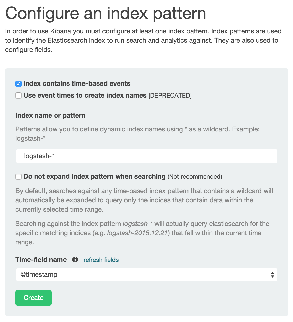
Access http://localhost:5601/ with a Web browser. Kibana is running correctly if it shows a page saying “Configure an index pattern”. Since Elasticsearch does not have any data yet, no more operation is necessary at the moment. In the Running SensorBee section further configuration steps are described.
1.2.2. Installation and Setup
At this point, the environment described in the previous section is assumed to be installed correctly and working. Now, some more components needs to be set up before continuing this tutorial.
1.2.2.1. Installing the Tutorial Package
To setting up the system, go get the tutorial package first:
$ go get github.com/sensorbee/tutorial/ml
The package contains configuration files in the config subdirectory
that are necessary for the tutorial. Create a temporary directory and copy those
files to the directory (replace /path/to/ with an appropriate path):
$ mkdir -p /path/to/sbml
$ cp -r $GOPATH/src/github.com/sensorbee/tutorial/ml/config/* /path/to/sbml/
$ cd /path/to/sbml
/path/to/sbml$ ls
Gemfile
build.yaml
fluent.conf
sensorbee.yaml
train.bql
twitter.bql
uds
1.2.2.2. Installing and Running fluentd
This tutorial, and SensorBee, relies on fluentd. fluentd is an open source data collector that provides many input and output plugins to connect with a wide variety of databases including Elasticsearch. Skip this subsection if fluentd is already installed.
To install fluentd for this tutorial, bundler needs to be installed with
the gem command. To see if it’s already installed, run gem list.
Something like bundler (1.11.2) shows up if it’s already installed:
/path/to/sbml$ gem list | grep bundler
bundler (1.11.2)
/path/to/sbml$
Otherwise, install bundler with gem install bundler. It may require admin
privileges (i.e. sudo):
/path/to/sbml$ gem install bundler
Fetching: bundler-1.11.2.gem (100%)
Successfully installed bundler-1.11.2
Parsing documentation for bundler-1.11.2
Installing ri documentation for bundler-1.11.2
Done installing documentation for bundler after 3 seconds
1 gem installed
/path/to/sbml$
After installing bundler, run the following command to install fluentd and its
plugins under the /path/to/sbml directory (in order to build the gems, you
may have to install Ruby header files before):
/path/to/sbml$ bundle install --path vendor/bundle
Fetching gem metadata from https://rubygems.org/............
Fetching version metadata from https://rubygems.org/..
Resolving dependencies...
Installing cool.io 1.4.3 with native extensions
Installing multi_json 1.11.2
Installing multipart-post 2.0.0
Installing excon 0.45.4
Installing http_parser.rb 0.6.0 with native extensions
Installing json 1.8.3 with native extensions
Installing msgpack 0.5.12 with native extensions
Installing sigdump 0.2.4
Installing string-scrub 0.0.5 with native extensions
Installing thread_safe 0.3.5
Installing yajl-ruby 1.2.1 with native extensions
Using bundler 1.11.2
Installing elasticsearch-api 1.0.15
Installing faraday 0.9.2
Installing tzinfo 1.2.2
Installing elasticsearch-transport 1.0.15
Installing tzinfo-data 1.2016.1
Installing elasticsearch 1.0.15
Installing fluentd 0.12.20
Installing fluent-plugin-elasticsearch 1.3.0
Bundle complete! 2 Gemfile dependencies, 20 gems now installed.
Bundled gems are installed into ./vendor/bundle.
/path/to/sbml$
With --path vendor/bundle option, all Ruby gems required for this tutorial
is locally installed in the /path/to/sbml/vendor/bundle directory. To
confirm whether fluentd is correctly installed, run the command below:
/path/to/sbml$ bundle exec fluentd --version
fluentd 0.12.20
/path/to/sbml$
If it prints the version, the installation is complete and fluentd is ready to be used.
Once fluentd is installed, run it with the provided configuration file:
/path/to/sbml$ bundle exec fluentd -c fluent.conf
2016-02-05 16:02:10 -0800 [info]: reading config file path="fluent.conf"
2016-02-05 16:02:10 -0800 [info]: starting fluentd-0.12.20
2016-02-05 16:02:10 -0800 [info]: gem 'fluentd' version '0.12.20'
2016-02-05 16:02:10 -0800 [info]: gem 'fluent-plugin-elasticsearch' version '1.3.0'
2016-02-05 16:02:10 -0800 [info]: adding match pattern="sensorbee.tweets" type="...
2016-02-05 16:02:10 -0800 [info]: adding source type="forward"
2016-02-05 16:02:10 -0800 [info]: using configuration file: <ROOT>
  <source>
    @type forward
    @id forward_input
  </source>
  <match sensorbee.tweets>
    @type elasticsearch
    host localhost
    port 9200
    include_tag_key true
    tag_key @log_name
    logstash_format true
    flush_interval 1s
  </match>
</ROOT>
2016-02-05 16:02:10 -0800 [info]: listening fluent socket on 0.0.0.0:24224
Some log messages are truncated with ... at the end of each line.
The configuration file fluent.conf is provided as a part of this tutorial.
It defines a data source using in_forward and a destination that
is connected to Elasticsearch. If the Elasticserver is running on a different
host or using a port number different from 9200, edit fluent.conf:
<source>
  @type forward
  @id forward_input
</source>
<match sensorbee.tweets>
  @type elasticsearch
  host {custom host name}
  port {custom port number}
  include_tag_key true
  tag_key @log_name
  logstash_format true
  flush_interval 1s
</match>
Also, feel free to change other parameters to adjust the configuration to the actual environment. Parameters for the Elasticsearch plugin are described at https://github.com/uken/fluent-plugin-elasticsearch.
1.2.2.3. Create Twitter API Key
This tutorial requires Twitter’s API keys. To create keys, visit Application Management. Once a new application is created, click the application and its “Keys and Access Tokens” tab. The page should show 4 keys:
- Consumer Key (API Key)
- Consumer Secret (API Secret)
- Access Token
- Access Token Secret
Then, create the api_key.yaml in the /path/to/sbml directory and copy
keys to the file as follows:
/path/to/sbml$ cat api_key.yaml
consumer_key: <Consumer Key (API Key)>
consumer_secret: <Consumer Secret (API Secret)>
access_token: <Access Token>
access_token_secret: <Access Token Secret>
Replace each key’s value with the actual values shown in Twitter’s application management page.
1.2.3. Running SensorBee
All requirements for this tutorial have been installed and set up. The next
step is to install build_sensorbee, then build and run the sensorbee
executable:
/path/to/sbml$ go get gopkg.in/sensorbee/sensorbee.v0/...
/path/to/sbml$ build_sensorbee
sensorbee_main.go
/path/to/sbml$ ./sensorbee run -c sensorbee.yaml
INFO[0000] Setting up the server context                 config={"logging":
{"log_dropped_tuples":false,"min_log_level":"info","summarize_dropped_tuples":
false,"target":"stderr"},"network":{"listen_on":":15601"},"storage":{"uds":
{"params":{"dir":"uds"},"type":"fs"}},"topologies":{"twitter":{"bql_file":
"twitter.bql"}}}
INFO[0000] Setting up the topology                       topology=twitter
INFO[0000] Starting the server on :15601
Because SensorBee loads pre-trained machine learning models on its startup,
it may take a while to set up a topology. After the server shows the
message Starting the server on :15601, access Kibana at
http://localhost:5601/. If the setup operations performed so far have been
successful, it returns the page as shown below with a green “Create” button:
(If the button is not visible, see the section on Troubleshooting below.) Click the “Create” button to work with data coming from SensorBee. After the action is completed, you should see a list of fields that were found in the data stored so far. If you click “Discover” in the top menu, a selection of the tweets and a diagram with the tweet frequency should be visible.
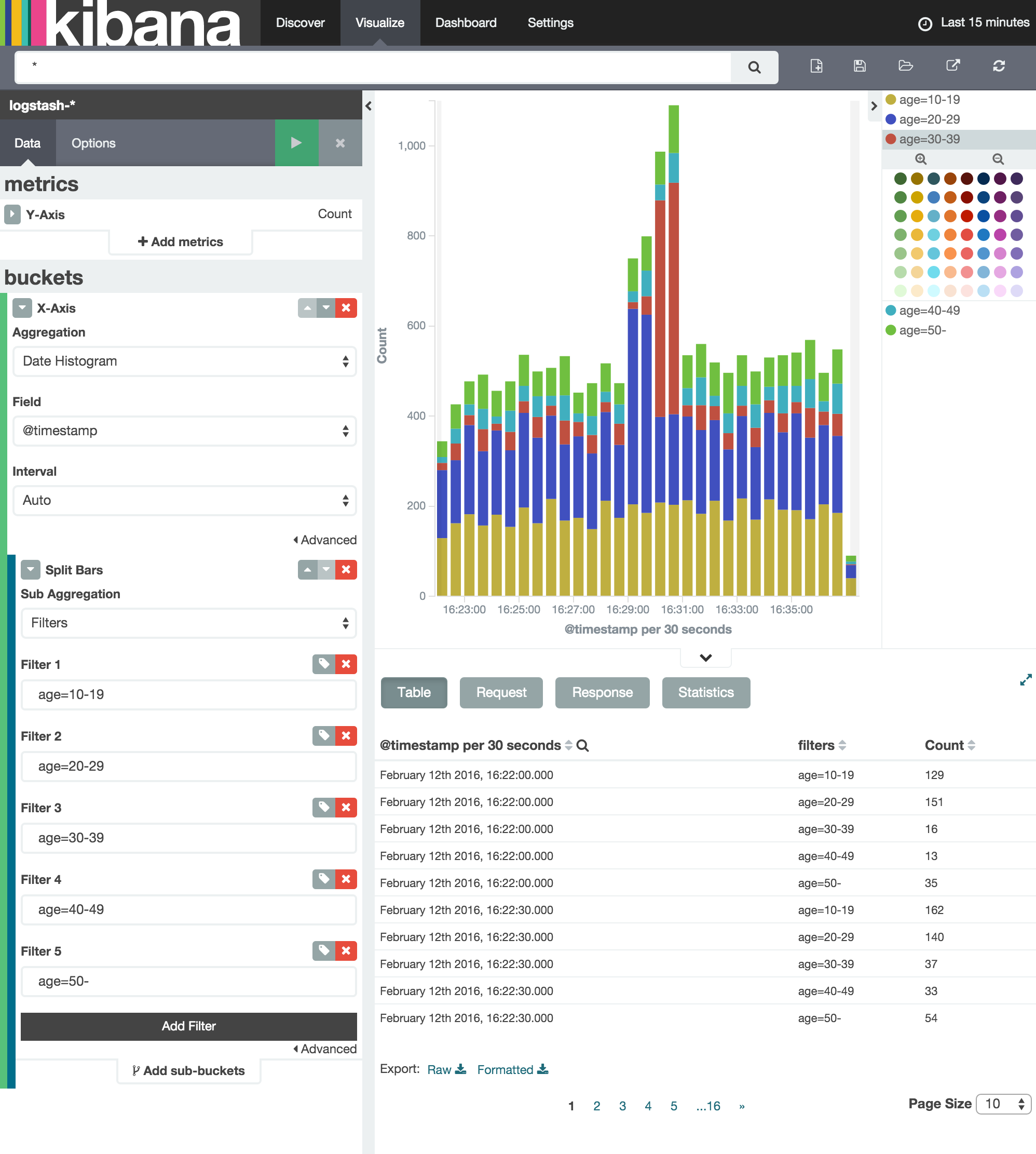
Kibana can now be used to visualize and search through the data in Elasticsearch. Although this tutorial doesn’t describe the usage of Kibana, many tutorials and examples can be found on the Web. The picture below shows an example chart showing some classification metrics:
1.2.3.1. Troubleshooting
If Kibana doesn’t show the “Create” button, something may not be working
properly. First, enter sensorbee shell to see SensorBee is working:
/path/to/sbml$ ./sensorbee shell -t twitter
twitter>
Then, issue the following SELECT statement:
twitter> SELECT RSTREAM * FROM public_tweets [RANGE 1 TUPLES];
... tweets show up here ...
If the statement returns an error or it doesn’t show any tweet:
- the host may not be connected to Twitter. Check the internet connection with
commands such as
ping. - The API key written in
api_key.yamlmay be wrong.
When the statement above shows tweets, query another stream:
twitter> SELECT RSTREAM * FROM labeled_tweets [RANGE 1 TUPLES];
... tweets show up here ...
If the statement doesn’t show any tweets, the format of tweets may have been
changed since the time of this writing. If so, modify BQL statements in
twitter.bql to support the new format. BQL Statements and Plugins
describes what each statement does.
When the statement above prints tweets, fluentd or Elasticsearch may have not been started yet. Check they’re running correctly.
For other errors, report them to https://github.com/sensorbee/tutorial.
1.2.4. BQL Statements and Plugins
This section describes how SensorBee produced the output that was
seen in the previous section: How it loads tweets from Twitter, preprocesses
tweets for machine learning, and finally classifies tweets to extract
demographic information of each tweets. twitter.bql in the config
directory contains all BQL statements used in this tutorial.
The following subsections explains what each statement does. To interact with some
streams created by twitter.bql, open another terminal (while the sensorbee
instance from the previous section is still running) and launch
sensorbee shell:
/path/to/sbml$ ./sensorbee shell -t twitter
twitter>
In the following sections of this tutorial, statements prefixed with
twitter> can be executed in the SensorBee shell; statements without this prefix
are statements from the twitter.bql file.
1.2.4.1. Creating a Twitter Source
This tutorial does not work without retrieving the public timeline of Twitter using the Sample API. The Sample API is provided for free to retrieve a portion of tweets sampled from the public timeline.
The github.com/sensorbee/twitter
package provides a plugin for public time line retrieval. The source provided by that plugin has the type
twitter_public_stream. The plugin can be registered to the SensorBee
server by adding github.com/sensorbee/twitter/plugin to the build.yaml
configuration file for build_sensorbee. Now consider the first statement
in the twitter.bql file:
CREATE SOURCE public_tweets TYPE twitter_public_stream
    WITH key_file = "api_key.yaml";
This statement creates a new source with the name public_tweets. To retrieve raw
tweets from that source, run the following SELECT statement in the
SensorBee shell:
twitter> SELECT RSTREAM * FROM public_tweets [RANGE 1 TUPLES];
Note
For simplicity, a relative path is specified as the key_file parameter.
However, it is usually recommended to pass an absolute path when
running the SensorBee server as a daemon.
1.2.4.2. Preprocessing Tweets and Extracting Features for Machine Learning
Before applying machine learning to tweets, they need to be converted into another form of information so that machine learning algorithms can utilize them. The conversion consists of two tasks: preprocessing and feature extraction. Preprocessing generally involves data cleansing, filtering, normalization, and so on. Feature extraction transforms preprocessed data into several pieces of information (i.e. features) that machine learning algorithms can “understand”.
Which preprocessing or feature extraction methods are required for machine learning varies depending on the format or data type of input data or machine learning algorithms to be used. Therefore, this tutorial only shows one example of applying a classification algorithm to English tweets.
Selecting Meaningful Fields of English Tweets
Because this tutorial aims at English tweets, tweets written in other
languages needs to be removed. This can be done with the WHERE
clause, as you can check in the SensorBee shell:
twitter> SELECT RSTREAM * FROM public_tweets [RANGE 1 TUPLES]
    WHERE lang = "en";
Tweets have the lang field and it can be used for the filtering.
In addition to it, not all fields in a raw tweet will be required for machine learning. Thus, removing unnecessary fields keeps data simple and clean:
CREATE STREAM en_tweets AS
    SELECT RSTREAM
        "sensorbee.tweets" AS tag, id_str AS id, lang, text,
        user.screen_name AS screen_name, user.description AS description
    FROM public_tweets [RANGE 1 TUPLES]
    WHERE lang = "en";
This statement creates a new stream en_tweets. It only selects English
tweets by WHERE lang = "en". "sensorbee.tweets" AS tag is used by
fluentd sink later. The items in that stream will look like:
{
    "tag": "sensorbee.tweets",
    "id": "the string representation of tweet's id",
    "lang": "en",
    "text": "the contents of the tweet",
    "screen_name": "user's @screen_name",
    "description": "user's profile description"
}
Note
AS in user.screen_name AS screen_name is required at the moment.
Without it, the field would have the name like col_n. This is because
user.screen_name could be evaluated as a JSON Path and might result in
multiple return values so that it cannot properly be named. This
specification might be going to be changed in the future version.
Removing Noise
Noise that is meaningless and could be harmful to machine learning algorithms needs to be removed. The field of natural language processing (NLP) has developed many methods for this purpose and they can be found in a wide variety of articles. However, this tutorial only applies some of the most basic operations on each tweets.
CREATE STREAM preprocessed_tweets AS
    SELECT RSTREAM
        filter_stop_words(
            nlp_split(
                nlp_to_lower(filter_punctuation_marks(text)),
            " ")) AS text_vector,
        filter_stop_words(
            nlp_split(
                nlp_to_lower(filter_punctuation_marks(description)),
            " ")) AS description_vector,
        *
    FROM en_tweets [RANGE 1 TUPLES];
The statement above creates a new stream preprocessed_tweets from
en_tweets. It adds two fields to the tuple emitted from en_tweets:
text_vector and description_vector. As for preprocessing, the
statement applies following methods to text and description fields:
- Remove punctuation marks
- Change uppercase letters to lowercase
- Remove stopwords
First of all, punctuation marks are removed by the user-defined function (UDF)
filter_puncuation_marks. It is provided in a plugin for this tutorial in the
github.com/sensorbee/tutorial/ml package. The UDF removes some punctuation
marks such as ”,”, ”.”, or “()” from a string.
Note
Emoticons such as ”:)” may play a very important role in classification
tasks like sentiment estimation. However, filter_punctuation_marks
simply removes most of them for simplicity. Develop a better UDF to solve
this issue as an exercise.
Second, all uppercase letters are converted into lowercase letters by
the nlp_to_lower UDF. The UDF is registered in
github.com/sensorbee/nlp/plugin. Because a letter is mere byte code and
the values of “a” and “A” are different, machine learning algorithms consider
“word” and “Word” have different meanings. To avoid that confusion, all letters
should be “normalized”.
Note
Of course, some words should be distinguished by explicitly starting with an uppercase. For example, “Mike” could be a name of a person, but changing it to “mike” could make the word vague.
Finally, all stopwords are removed. Stopwords are words that appear too often
and don’t provide any insight for classification. Stopword filtering in this
tutorial is done in two steps: tokenization and filtering. To perform a
dictionary-based stopword filtering, the content of a tweet needs to be
tokenized. Tokenization is a process that converts a sentence into a sequence
of words. In English, “I like sushi” will be tokenized as
["I", "like", "sushi"]. Although tokenization isn’t as simple as just
splitting words by white spaces, the preprocessed_tweets stream simply
does it for simplicity using the UDF nlp_split, which is defined in the
github.com/sensorbee/nlp package. nlp_split takes two arguments: a
sentence and a splitter. In the statement, contents are split by a white
space. nlp_split returns an array of strings. Then, the UDF
filter_stop_words takes the return value of nlp_split and removes
stopwords contained in the array. filter_stop_word is provided as a part
of this tutorial in the github.com/sensorbee/tutorial/ml package. It’s a mere
example UDF and doesn’t provide perfect stopword filtering.
As a result, both text_vector and description_vector have an array
of words like ["i", "want", "eat", "sushi"] created from the sentence
I want to eat sushi..
Preprocessing shown so far is very similar to the preprocessing required for full-text search engines. There should be many valuable resources among that field including Elasticsearch.
Note
For other preprocessing approaches such as stemming, refer to natural language processing textbooks.
Creating Features
In NLP, a bag-of-words representation is usually used as a feature for machine learning algorithms. A bag-of-words consists of pairs of a word and its weight. Weight could be any numerical value and usually something related to term frequency (TF) is used. A sequence of the pairs is called a feature vector.
A feature vector can be expressed as an array of weights. Each word in all tweets observed by a machine learning algorithm corresponds to a particular position of the array. For example, the weight of the word “want” may be 4th element of the array.
A feature vector for NLP data could be very long because tweets contains many words. However, each vector would be sparse due to the maximum length of tweets. Even if machine learning algorithms observe more than 100,000 words and use them as features, each tweet only contains around 30 or 40 words. Therefore, each feature vector is very sparse, that is, only a small number its elements have non-zero weight. In such cases, a feature vector can effectively expressed as a map:
{
    "word": weight,
    "word": weight,
    ...
}
This tutorial uses online classification algorithms that are imported from Jubatus, a distributed online machine learning server. These algorithms accept the following form of data as a feature vector:
{
    "word1": 1,
    "key1": {
        "word2": 2,
        "word3": 1.5,
    },
    "word4": [1.1, 1.2, 1.3]
}
The SensorBee terminology for that kind of data structure is “map”. A map can be nested and its value can be an array containing weights. The map above is converted to something like:
{
    "word1": 1,
    "key1/word2": 2,
    "key1/word3": 1.5,
    "word4[0]": 1.1,
    "word4[1]": 1.2,
    "word4[2]": 1.3
}
The actual feature vectors for the tutorial are created in the fv_tweets
stream:
CREATE STREAM fv_tweets AS
  SELECT RSTREAM
    {
        "text": nlp_weight_tf(text_vector),
        "description": nlp_weight_tf(description_vector)
    } AS feature_vector,
    tag, id, screen_name, lang, text, description
FROM preprocessed_tweets [RANGE 1 TUPLES];
As described earler, text_vector and description_vector are arrays of
words. The nlp_weight_tf function defined in the github.com/sensorbee/nlp
package computes a feature vector from an array. The weight is term
frequency (i.e. the number of occurrences of a word). The result is a map
expressing a sparse vector above. To see how the feature_vector looks
like, just issue a SELECT statement for the fv_tweets stream.
All required preprocessing and feature extraction have been completed and it’s now ready to apply machine learning to tweets.
1.2.4.3. Applying Machine Learning
The fv_tweets stream now has all the information required by a machine
learning algorithm to classify tweets. To apply the algorithm for each tweets,
pre-trained machine learning models have to be loaded:
LOAD STATE age_model TYPE jubaclassifier_arow
    OR CREATE IF NOT SAVED
    WITH label_field = "age", regularization_weight = 0.001;
LOAD STATE gender_model TYPE jubaclassifier_arow
    OR CREATE IF NOT SAVED
    WITH label_field = "gender", regularization_weight = 0.001;
In SensorBee, machine learning models are expressed as user-defined states
(UDSs). In the statement above, two models are loaded: age_model and
gender_model. These models contain the necessary information to classify gender and
age of the user of each tweet. The model files are located in the uds directory
that was copied from the package’s config directory beforehand:
/path/to/sbml$ ls uds
twitter-age_model-default.state
twitter-gender_model-default.state
These filenames were automatically assigned by SensorBee server when the
SAVE STATE statement was issued. It will be described later.
Both models have the type jubaclassifier_arow imported from
Jubatus. The UDS type is implemented in the
github.com/sensorbee/jubatus/classifier
package. jubaclassifier_arow implements the AROW online linear classification
algorithm [Crammer09]. Parameters specified in the WITH clause are related
to training and will be described later.
After loading the models as UDSs, the machine learning algorithm is ready to work:
CREATE STREAM labeled_tweets AS
    SELECT RSTREAM
        juba_classified_label(jubaclassify("age_model", feature_vector)) AS age,
        juba_classified_label(jubaclassify("gender_model", feature_vector)) AS gender,
        tag, id, screen_name, lang, text, description
    FROM fv_tweets [RANGE 1 TUPLES];
The labeled_tweets stream emits tweets with age and gender labels.
The jubaclassify UDF performs classification based on the given model.
twitter> EVAL jubaclassify("gender_model", {
    "text": {"i": 1, "wanna": 1, "eat":1, "sushi":1},
    "description": {"i": 1, "need": 1, "sushi": 1}
});
{"male":0.021088751032948494,"female":-0.020287269726395607}
jubaclassify returns a map of labels and their scores as shown above. The
higher the score of a label, the more likely a tweet has the label. To choose
the label having the highest score, the juba_classified_label function is
used:
twitter> EVAL juba_classified_label({
    "male":0.021088751032948494,"female":-0.020287269726395607});
"male"
jubaclassify and juba_classified_label functions are also defined in
the github.com/sensorbee/jubatus/classifier package.
| [Crammer09] | Koby Crammer, Alex Kulesza and Mark Dredze, Adaptive Regularization Of Weight Vectors, Advances in Neural Information Processing Systems, 2009 |
1.2.4.4. Inserting Labeled Tweets Into Elasticsearch via Fluentd
Finally, tweets labeled by machine learning need to be inserted into Elasticsearch for visualization. This is done via fluentd which was previously set up.
CREATE SINK fluentd TYPE fluentd;
INSERT INTO fluentd from labeled_tweets;
SensorBee provides fluentd plugins in the github.com/sensorbee/fluentd
package. The fluentd sink write tuples into fluentd’s forward input
plugin running on the same host.
After creating the sink, the INSERT INTO statement starts writing tuples
from a source or a stream into it. This statement is the last one in the
twitter.bql file and also concludes this section. All the steps from
connecting to the Twitter API, transforming tweets and analyzing them using
Jubatus have been shown in this section. As the last part of this tutorial,
it will be shown how the training of the previously loaded model files has
been done.
1.2.5. Training
The previous section used the machine learning models that were already trained
but it was not described how to train them. This section explains how machine
learning models can be trained with BQL and the sensorbee command.
1.2.5.1. Preparing Training Data
Because the machine learning algorithm used in this tutorial is supervised learning, it requires a training data set to create models. Training data is a pair of original data and its label. There is no common format of a training data set and a format can vary depending on use cases. In this tutorial, a training data set consists of multiple lines each of which has exactly one JSON object.
{"description":"I like sushi.", ...}
{"text":"I wanna eat sushi.", ...}
...
In addition, each JSON object needs to have two fields “age” and “gender”:
{"age":"10-19","gender":"male", ...other original fields...}
{"age":"20-29","gender":"female", ...other original fields...}
...
In the pre-trained model, age and gender have following labels:
age
10-1920-2930-3940-4950<
gender
malefemale
Both age and gender can have additional labels if necessary. Labels can be empty
if they are not known for sure. After annotating each tweet, the training data set needs
to be saved as training_tweets.json in the /path/to/sbml directory.
The training data set used for the pre-trained models contains 4974 gender labels and 14747 age labels.
1.2.5.2. Training
Once the training data set has been prepared, the models can be trained with the following command:
/path/to/sbml$ ./sensorbee runfile -t twitter -c sensorbee.yaml -s '' train.bql
sensorbee runfile executes BQL statements written in a given file,
e.g. train.bql in the command above. -t twitter means the name of the
topology is twitter. The name is used for the filenames of saved models
later. -c sensorbee.yaml passes the same configuration file as the one
used previously. -s '' means sensorbee runfile saves all UDSs after the
topology stops.
After running the command above, two models (UDSs) are saved in the uds
directory. The saved model can be loaded by the LOAD STATE statement.
1.2.5.3. BQL Statements
All BQL statements for training are written in train.bql. Most statements
in the file overlap with twitter.bql, so only differences will be explained.
CREATE STATE age_model TYPE jubaclassifier_arow
    WITH label_field = "age", regularization_weight = 0.001;
CREATE SINK age_model_trainer TYPE uds WITH name = "age_model";

CREATE STATE gender_model TYPE jubaclassifier_arow
    WITH label_field = "gender", regularization_weight = 0.001;
CREATE SINK gender_model_trainer TYPE uds WITH name = "gender_model";
These statements create UDSs for machine learning models of age and gender
classifications. CREATE STATE statements are same as ones in
twitter.bql. The CREATE SINK statements above create new sinks with the
type uds. The uds sink writes tuples into the UDS specified as name if the UDS
supports it. jubaclassifier_arow supports writing tuples. When a tuple is
written to it, it trains the model with the tuple having training data. It
assumes that the tuple has two fields: a feature vector field and a label field.
By default, a feature vector and a label are obtained by the feature_vector
field and the label field in a tuple, respectively. In this tutorial, each
tuple has two labels: age and gender. Therefore, the field names of
those fields need to be customized. The field names can be specified by the
label_field parameter in the WITH clause of the CREATE STATE
statement. In the statements above, age_model and gender_model UDSs
obtain labels from the age field and the gender field, respectively.
CREATE PAUSED SOURCE training_data TYPE file WITH path = "training_tweets.json";
This statement creates a source which inputs tuples from a file.
training_tweets.json is the file prepared previously and contains training
data. The source is created with the PAUSED flag, so it doesn’t emit any
tuple until all other components in the topology are set up and the
RESUME SOURCE statement is issued.
en_tweets, preprocessed_tweets, and fv_tweets streams are same as
ones in twitter.bql except that the tweets are emitted from the file source
rather than the twitter_public_stream source.
CREATE STREAM age_labeled_tweets AS
    SELECT RSTREAM * FROM fv_tweets [RANGE 1 TUPLES] WHERE age != "";
CREATE STREAM gender_labeled_tweets AS
    SELECT RSTREAM * FROM fv_tweets [RANGE 1 TUPLES] WHERE gender != "";
These statements create new sources that only emit tuples having a label for training.
INSERT INTO age_model_trainer FROM age_labeled_tweets;
INSERT INTO gender_model_trainer FROM gender_labeled_tweets;
Then, those filtered tuples are written into models (UDSs) via the uds sinks
created earlier.
RESUME SOURCE training_data;
All streams are set up and the training_data source is finally resumed.
With the sensorbee runfile command, all statements run until all tuples
emitted from the training_data source are processed.
When BQL statements are run on the server, the SAVE STATE statement is
usually used to save UDSs. However, sensorbee runfile optionally saves UDSs
after the topology is stopped. Therefore, train.bql doesn’t issue
SAVE STATE statements.
1.2.5.4. Evaluation
Evaluation tools are being developed.
1.2.5.5. Online Training
All machine learning algorithms provided by Jubatus are online algorithms, that is, models can incrementally be trained every time a new training data is given. In contrast to online algorithms, batch algorithms requires all training data for each training. Since online machine learning algorithms don’t have to store training data locally, they can train models from streaming data.
If training data can be obtained by simple rules, training and classification can be applied to streaming data concurrently in the same SensorBee server. In other words, a UDS can be used for training and classification.